Introduction

Medical decision making is supported by pharmacoeconomic analyses, which are usually based on modeling of health effects and costs. A common tool used in such analyses are Markov models, which enable the progress of the diseases to be simulated throughout the lifetime of patients [1,2]. One of the problems that arise whilst modeling long-term costs and health outcomes utilizing Markov models is the choice of transition time between health states. Once a specific cycle length is adopted, it allows to change the status of disease (progression, regression or death) only at specific time points, which does not always adequately reflect the course of disease in real life [1]. Various approaches can be adopted, i.e. transitions at the beginning or at the end of the cycle and more accurate methods like half-cycle correction (HCC), ‘life-table’ method (LT), or Simpson’s method [3,4]. The half-cycle correction and the ‘life-table’ method are equivalent in some situations: if costs/utilities are equal in each cycle and there is no discounting [4]. Despite some limitations [4,5], the most common method used in economic evaluations, which is also recommended by some of national HTA agencies [6–9], is half-cycle correction.

The practical implementation of the half-cycle correction and ‘life-table’ method has been described in other publications [1,4].

Our aim is to review information concerning various approaches to choosing time of transition, accuracy of these methods and to establish whether there is an optimal cycle length for which HCC/LT should always be applied.

Methods

We developed a simple two-state Markov model (alive or dead) in order to analyze the influence of cycle length on differences between analyzed methods.

The time horizon was set to be lifetime, the discount rate was 0–5% and costs/utilities were held constant in time.

Assuming different death probabilities (0.05–0.90 annually), we compared four approaches:

• transitions at the beginning of the cycle (‘beginning’),
• transitions at the end of the cycle (‘end’),
• half-cycle correction,
• ‘life-table’ method.

Half-cycle correction is made to transitions either at the beginning or at the end of the cycle. The method of calculations differs slightly between those two assumptions, however in both cases identical results are obtained. In case of progression at the end of the cycle, HCC is implemented by cutting off the first half of the first cycle. If the horizon of the analysis is shorter than lifetime, patient/cohort’s life must be modeled one cycle longer then the assumed time horizon and the results for the first half of the additional cycle must be added to cumulative results. In case of progression at the beginning of the cycle, HCC is implemented by adding half of a cycle at the beginning of the analysis. If the horizon of the analysis is shorter than lifetime, this action will result in overestimation of the results, therefore, an additional correction must be made by cutting off second half of the last cycle.

Both of the described methods result in the same final outcomes, so we use the same outcomes for HCC when comparing it with both ‘beginning’ and ‘end’ methods.

The ‘life-table’ method is implemented by calculating number of patients staying in particular state as a mean number of patients staying in this state at the beginning and at the end of the cycle (arithmetic mean, i.e. assuming linear progression).

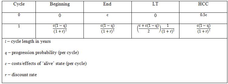
The key issue concerned with the use of different methods is establishing the time points when costs/health effects are calculated (discounting time). For ‘beginning’ and LT method we assumed that there are no costs/effects incurred in cycle 0 (cycle, in which no discounting is applied). For ‘end’ method we assigned full cost to the cycle 0 and for HCC method we assigned half of these costs to the cycle 0 (Table 1). Such procedure is coherent with practical approach in pharmacoeconomic models.

Table 1. Amount of costs/health effects in cycle 0 and 1

We assumed progression probabilities to be constant in time. For each probability the threshold values were determined, i.e. the maximal cycle lengths for which the differences between half-cycle correction/’life-table’ method and ’beginning’/‘end’ methods were not greater than 5%. We propose that cycles longer than the estimated threshold should imply the application of HCC/LT.

Furthermore, influence of applied assumptions (cost/utilities and death probabilities variability, number of health states in the model) on the obtained results and consequences of relaxing them were analyzed. Additionally, we studied the relationship between threshold cycle lengths and incremental results, and made an attempt to provide general conclusions concerning incremental cost-effectiveness ratios (ICERs).

All calculations were performed using Microsoft Excel® 2007.

Results

General relations between cycle length, death probability and the method of calculation

The problem of calculating costs / health effects for a cohort of patients may be illustrated by graphs which link survival curves with costs/utilities. Such graphs may be created for every state, however in more complicated models this is an incredibly laborious task. The final result (i.e. total costs, expected survival) would be the sum of areas under the curves.

A mathematical approach to the problem of calculating the area under the curve would be solving a corresponding integral. When discrete Markov models are used, the approximate area is calculated as the sum of areas of respective rectangles. All four methods (‘beginning’, ‘end’, HCC, LT) provide approximate outcomes, which become more accurate as smaller rectangles are used. Using Markov models language, it means that the shorter cycle is chosen, the more accurate outcomes are obtained. It is intuitive: if a short cycle is used, we are able to describe more precisely the moments of transitions between states. The illustrative results for probability of death equal to 0.5 are presented on Figure 1.

Figure 1. Comparison of differences in total costs between methods for various cycle lengths

Assumptions: progression rate – 0.5, annual cost for ‘alive’ state – 200, annual cost for death state – 0, discount rate 5%.
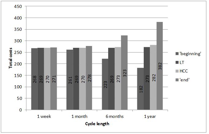
The exact result (calculated using integrals) is 269.56.

 

If the horizon of analysis is finite (i.e. not lifetime), the accuracy of the approximation depends also on the slope of the curve (progression probabilities in Markov models). The steeper the slope, the less precise the approximation of the area (results for several slopes are presented on Figure 2).

Figure 2.Compariso n of differences in total costs between methods for various progression rates

                                                                                                                                                               Assumptions: horizon 5 years, cycle length 1 year, annual costs 200, discount rate 5%.
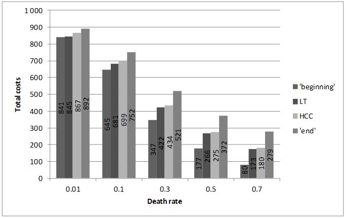
The exact results (obtained using integrals) are 866.32, 697.16, 428.30, 262.96, 159.34 .for rates 0.01, 0.1, 0.3, 0.5, 0.7, respectively

In case of lifetime horizon the differences between ‘beginning’, ‘end’ and HCC methods are associated with the differences in approach to cycle 0. As a result, the difference between results obtained using different methods is equal to the difference obtained in cycle 0 and does not depend on the progression probability (provided it is constant). However, the percentage difference between results obtained using HCC and ‘beginning’ / ‘end’ methods depends on the probability because the total outcomes are strictly related to the probability of transition. For example, assuming annual costs of ‘alive’ state equal to 200, discount rate 5%  and progression probabilities equal to 0.7 or 0.8 the differences between total outcomes for HCC and other methods are 100 for both probabilities of death and the percentage differences are 56% and 68% for probabilities 0.7 and 0.8, respectively.

As far as LT method is concerned, the difference between total results for this method and for ‘beginning’ / ‘end’ is associated not only with cycle 0, but also with other cycles. Moreover, the percentage differences for LT vs ‘beginning’ method and LT vs ‘end’ method are in general not equal.

However, it may be easily shown that percentage differences between costs/effects for LT and ‘beginning’ / ‘end’ method in any single cycle are constant and, as a result, equal to the percentage differences for total costs/effects (Table 2).

Table 2. Percentage differences in single cycle results between LT and ‘beginning’ / ‘end’ methods

                                                                                                                                                                                                                                                                            The same results may be obtained for any other cycle.

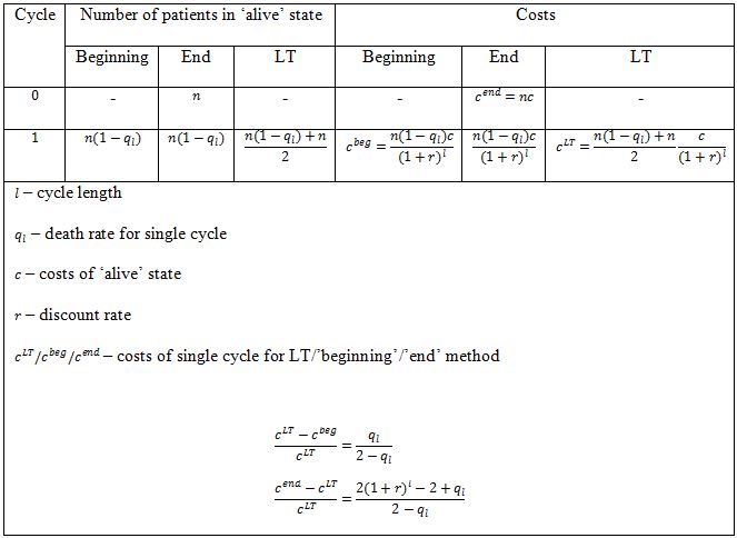
The percentage differences between results obtained using different methods do not depend on the magnitude of costs / health effects. In the example described above annual costs of the ‘alive’ state were assumed to be 200; however, under the assumptions made previously, any other cost would provide the same results for percentage differences. Therefore the results described further are general, and the only important assumptions are two-state model and constancy of costs/utilities and progression probabilities in time.

Threshold cycle lengths depending on death probabilities

In Table 3 threshold cycle lengths for various transition probabilities are presented. The threshold was defined as the cycle length for which the difference between HCC and ‘beginning’ / ‘end’ methods is equal to 5% or the cycle length for which the maximum of differences between LT and ‘beginning’ / ‘end’ methods is equal to 5%. Following the results obtained earlier, adopting the cycle length shorter than the threshold provides results which differ by less than 5% (more accurate approximation). Differences between HCC and ‘beginning’ / ‘end’ methods do not depend on the discount rate (in lifetime horizon). However, the relative difference is smaller if lower discount rate is used. As a result, if the discount rate is lower, the threshold cycle length will be longer. For LT method, both differences and relative differences depend on discount rate (as a result of calculation in Table 2).

Table 3. Threshold cycle lengths depending on progression rate

*) assumptions: discount rate – 5%, initial age – 50
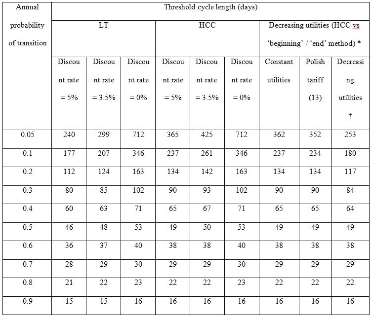
†) for age ≥ 55 utility equal to 0.5

Threshold cycle lengths for costs/utilities that are not constant

Costs/utilities are often not constant in time [10–12]. In Table 3 the comparison of threshold cycle lengths is presented for HCC for constant utilities and utilities depending on age (using the age-specific multipliers according to Polish tariff [13] and hypothetical 50% decrease of utility at the age of 55). As expected, the thresholds for decreasing utilities are slightly lower, the largest differences are observed for the slowest progression probabilities. Similar results and dependencies may be obtained for LT method.

Incremental results

The challenging problem to determine the threshold cycle length occurs also when investigating incremental outcomes. The key issue is the fact that there are differences between two interventions associated with progression probabilities and cost/utilities varying over time. Concluding from what was shown before, when the outcomes are calculated for single intervention the costs/utilities of health states do not influence the percentage differences between methods. However, if incremental results are calculated, the total amount of costs / health effects for separate interventions is crucial and therefore any change of the cost/utility of health state results in changes in incremental costs/effects. For example, assuming 1 month cycle, death probability – 0.5 for intervention, and 0.7 for comparator, discount rates – 5% for costs and 3.5% for utilities and utility of ‘alive’ state – 0.85 we obtain following percentage differences between ICERs (HCC vs ‘beginning’ / ‘end’):

• 2.2% for annual costs of intervention and comparator equal to 400 and 200, respectively,
• 2.7% for annual costs of intervention and comparator equal to 700 and 200, respectively,
• 1.0% for annual costs of intervention and comparator equal to 700 and 600, respectively.

 However, in case of comparison of HCC and ‘beginning’ / ‘end’ methods, after making a few assumptions, it is possible to observe some general conclusions for ICER calculation. Suppose that a new treatment option is to be compared with standard practice (we will refer to them as intervention vs. comparator). We assume that:

1. the initial cohort distribution among health states and the utilities for each health state are the same for both options,
2. probability of death (progression) is lower for assessed intervention than for the comparator,
3. annual costs of health states for assessed intervention are higher than annual costs of the states for comparator.

The first assumption implies that incremental QALY (quality-adjusted life years) will be the same for all three methods [14]. The second assumption implies that the percentage difference between costs of intervention for analyzed methods is lower than the respective difference for comparator. Under these assumptions the percentage difference between ICERs obtained using the analyzed methods is not higher than the minimum of two percentage differences between total costs: for the intervention and for the comparator (Table 4).

Table 4. Percentage difference between ICERs obtained from HCC and ‘beginning’ method

The same results may be obtained for comparison between HCC and ‘end’ method.

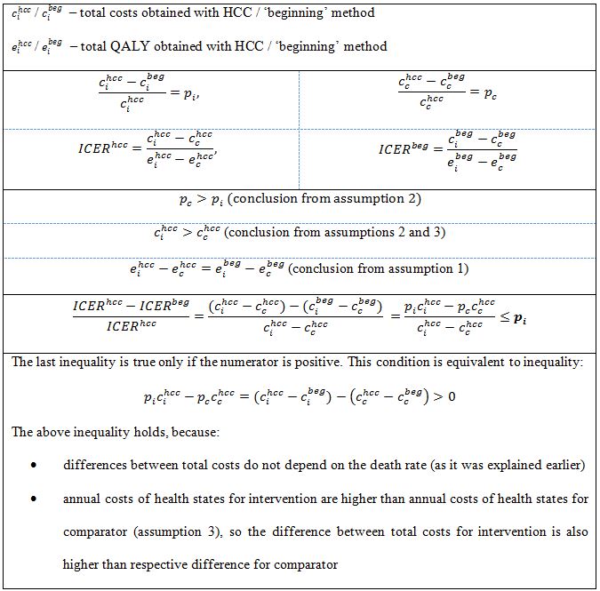
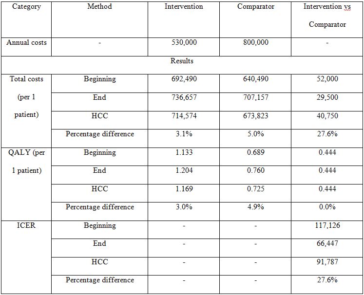
If annual costs of health states for the intervention are lower than annual costs for the comparator (assumption 3 is not satisfied) the last inequality from Table 4 does not hold and the previously made conclusion about ICERs is not true. However, if assumption 3 is not satisfied and annual costs of health states for the intervention are low enough to make the total costs of intervention be lower than total costs of comparator (by balancing the additional costs associated with lower progression probability), the ICERs are negative. In this case intervention dominates the comparator and there is no point in analyzing percentage differences between them. If the total costs of intervention remain higher than total costs of comparator, the percentage difference between ICERs may become large even in case of low percentage differences between costs. The example of such situation is presented in Table 5. The difference between ICERs for HCC and other methods is 27.6%, despite the difference between total costs being not higher than 5%.

Table 5. Large difference between ICERs for specific costs data

Assumptions: 1 month cycle, probability of transition – 0.5 for intervention, 0.68 for comparator, discount rates – 5% for costs, 3.5% for utilities, utility of ‘alive’ state – 0.85

Generally, the smaller the difference between total costs of intervention and comparator, the higher the difference between ICERs, namely when

 

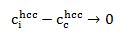
 then the percentage difference between ICERs increases rapidly:

 

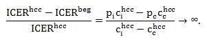
The results obtained for incremental results for HCC cannot be easily generalized for LT method, as the assumption of the same initial cohort distribution among health states and the same utilities for each health state for both options does not imply that incremental QALY will be the same for LT and ‘beginning’ / ‘end’ method.

Discussion

There is no general rule concerning the necessity of using half-cycle correction depending on cycle length. The ISPOR Good Research Practice recommend applying HCC in all cost-effectiveness analyses [15]. The guidelines provided by HTA agencies which mention this method do not precisely state when HCC should be used [6–9]. Therefore various approaches are adopted in economic analyses [16–19].

For a simple, 2-state Markov model it seems that in case of 2-week cycles or shorter half-cycle correction is unnecessary. The cycles shorter than thresholds result in differences between methods of less than 5%, which seems not to have significant impact on final results.

However the results were obtained under few assumptions:

• costs/utilities constant in time,
• progression probabilities constant in time,
• 2-state Markov model.

It is more difficult to calculate the threshold cycle lengths if some of the assumptions are not satisfied. However, it is possible to determine roughly the behavior of thresholds in cases where there are some variations in assumptions.

Costs/utilities are often not constant in time, e.g. utilities may depend on age. In case of relationships between HCC and ‘beginning’ / ‘end’ methods: if the costs/utilities decrease/increase, the total outcomes also decrease/increase and as a result the percentage differences increase/decrease which makes the thresholds lower/higher. If the changes are irregular, no general rule may be concluded. The highest variations, comparing with results for constant cots/utilities values, were observed for lower death probabilities. Furthermore, in practice progression probabilities are almost never constant. In case of relationships between HCC and ‘beginning’ / ‘end’ methods: if a probability of transition to state which is cheaper (or has lower utility) increases in time, the total results decrease and as a result the percentage differences increase which makes the thresholds lower. Similar conclusions can be made for opposite situations and LT method. Usually models consist of more than two states and some probabilities increase and other decrease. In such situations no general rule may be concluded.

If the model consists of more than two states it is difficult to make general conclusions about threshold cycle lengths. In order to make general rules, all possibilities of transitions between states should be analyzed and it would be complicated for multi-state models. When economic evaluations of health technologies are conducted, the key outcomes are usually ICERs and budget impact. Calculating the threshold cycle lengths for ICERs is a challenging problem. We made an attempt to analyze the relationship between threshold cycle lengths obtained for single interventions and the percentage differences between ICERs obtained using different methods. We showed that under a few assumptions, the percentage difference between ICERs obtained using different methods is not higher than the respective percentage differences between total costs for two compared interventions. However, there are situations when, despite low differences between total costs, the differences between ICERs are considerably high.

All the calculations and conclusions were made for lifetime horizon. However, if all the assumptions made at the beginning are satisfied, the results may be generalized for finite horizon models.

We did not identify other researches concerning the problem of conditions under which half-cycle should always be applied. Naimark et. al. [20] provided an explanation of half-cycle correction method. However, the authors did not make any specific recommendation when the correction should be used. Barendregt [4] outlined a few limitations of the method and suggested ‘life-table’ as alternative approach to be used in economic modeling. Another solution was suggested by Taylor et. al. [5], namely choosing as a time of transition the moment when half of the events occurs in each cycle. The authors indicated also the situations when the half-cycle correction use would not be justified, e.g. when patients use drugs which are bought at the beginning of cycles.

The main limitation of the study is a set of assumptions adopted in order to determine threshold cycle lengths. The set is very rarely satisfied in practice. However, skipping any of the assumptions significantly complicates the calculations and an appreciable number of possibilities need to be analyzed. An attempt was made to provide some general effects associated with relaxing some of assumptions as a pragmatic way forward.

Another limitation is applying the half-cycle correction to all costs/utilities in model. It is not always justified, e.g. there exists some costs that are incurred at the beginning of each period [5].

Conclusions

Choice of the time of transitions in the model may have a significant impact on results. For cycles shorter than 2 weeks HCC/LT method does not seem to be necessary. However, HCC/LT method should always be applied for cycles longer than 1 year. For cycles between 2 weeks and 1 year, we were unable to make a general recommendation.

Corresponding author:

Robert Drzal

HTA Consulting

ul. Starowiślna 17/3

31-038 Kraków

tel. (+48 12) 421-88-32

fax. (+48 12) 395-38-32

e-mail: office@hta.pl

Funding sources: The study received no external funding

Conflict of interest: no conflict of interest was identified